By Nicholas Guttenberg
Cross Compass
GoodAI
Summary
- How can we make an agent that can learn to perform a variety of tasks during its lifetime without being pre-trained on those tasks?
- The problem of expressivity: can we ensure that the solution to any task can be represented in some way that the agent (e.g. Badger) can ‘read’ and ‘execute’ in order to deploy that solution?
- We find that randomly initialized neural networks don’t capture a wide enough range of behaviors.
- However, if we use ‘mental affordances’ that ask for a network’s input/output relationships to be as diverse as possible, this increases the expressivity significantly.
- In the end this isn’t enough to encode solutions to complex tasks (like Atari games), suggesting we need further steps such as making the task codes modular.
- This suggests that task encodings within a modular agent (e.g. Badger architecture) likely need to be spread between modules rather than a one-module-per-task type of encoding.
You can find the code used to generate the results on GitHub here.
Introduction
The idea of the Badger architecture (https://arxiv.org/abs/1912.01513) is to make a learning agent with increased generality by virtue of allowing task-specific learning to occur in the activations of an extensible pool of ‘experts’ who all share the same weights. This in principle could avoid issues with catastrophic forgetting and improve both transfer and scalability. That is to say, if we use gradient descent to train a network on one task, and then another, then often the network forgets how to perform the first task. Badger’s approach to resolving this is similar in spirit to PathNet (https://arxiv.org/abs/1701.08734), which freezes the weights learned on one task and dynamically grows the network in weight space, using evolution to figure out which subsets of the network to engage. In the case of Badger, by comparison, the experts can be freely varied in number during inference or even in principle swapped back and forth between independent agents, and the experts themselves decide which other experts to connect to in trying to solve a particular task (via attention, for example).
But, is it possible to represent the solutions to every task that the (general) Badger agent might encounter in its runtime by sets of activations, rather than weights? Representing tasks as learned weights means operating in a space with a parameter count that is proportional to the square of the input, output, (and hidden) sizes — O(N²). Representing the same behaviors as activations reduces this to an O(N) parameter space (though if one task does not strictly correspond to one expert, this could be a larger space due to the number of experts). So as we move forward, it’s important to understand how expressive ‘representing learned behaviors as activation patterns’ is, compared to representing the same thing as weights.
It is also not clear how task-specific versus task-general knowledge would break down between different experts when training a Badger agent. If the experts are very powerful networks, then it is possible that gradient descent on the whole architecture will simply encode the solution for every task in the curriculum directly into the expert weights. It could also be that even if the expert weights encode a learning policy rather than a solving policy, the resultant expert activations might not encode representations of learned skills that are transferrable or generalizable across tasks.
This is made even more complicated by the fact that whatever online or recurrent computations need be done by the Badger agent in the process of solving a task will share the same space of activations as any information which is meant to persist between tasks. For some architectures, this may cause interference — the same kind of issue as the catastrophic forgetting that we wanted this approach to solve in the first place.
So in order to better understand the different possibilities, we consider the case in which we make an explicit separation not just into weights and activations, but into the following components:
- A ‘task encoding’ z which should vary only slowly during a task, but varies quickly between tasks.
- A network parameterized by weights W responsible for looking at the sensor inputs x, actions a, and results x′, and inferring a ‘task encoding’ that represents the task out of the ensemble of possible tasks: z = f ({x, x′, a}, W)
- A ‘scratch space’ h of fast activations which can vary quickly within a task and are used to perform the actual computation needed.
- A network parameterized by weights Φ which maps the combination of sensor inputs x, scratch space h, and task encoding z into new values of the scratch space h′ and actions a: h′ , a = g(x,h,z,Φ).
If we represent the Badger agent in this way, it breaks down the general problem of ‘meta-train to be able to learn new tasks during the agent’s lifetime’ into:
- (Somehow) determine a good network Φ
- For each task in the curriculum, (somehow) discover its appropriate task encoding(s) z.
- Train W to map sensory impressions to a distribution over z via gradient descent.
In terms of the Badger experts, each expert instantiates both a Φ and W network — the expert uses the information that is transmitted to it in the architecture to figure out what it should be doing (take up a z value for that task). So the difference between a dense network and a Badger agent would be, the dense network represents tasks as a single code vector whereas the Badger agent represents tasks as a collection of code vectors that each implement distinct sub-policies.
So, how do we do this?
The third of these steps is straightforward given the other two — it’s just a usual supervised learning problem. The second step would normally be hard, except that the parameter count of z can actually be much smaller than the parameter count of a full neural network. There’s a hint that this kind of policy compression can be successful in the results of the World Models study (https://arxiv.org/abs/1803.10122). In that study, given a strong sensory network to represent world states and a predictive network capable of representing state transitions, good policies could be discovered via evolution on extremely small neural networks. So in our case, it may indeed be feasible to discover policies via (for example) applying CMA-ES (see e.g. https://arxiv.org/abs/1604.00772) to a policy space of dimension <1000.
The issue then is, how to determine Φ?
Results from reservoir computing and echo state networks (see e.g. https://arxiv.org/abs/1712.04323) suggest that a random network may be sufficient to produce a large bank of potential dynamical behaviors. In those architectures, a final linear layer is trained to map from the space of random dynamics into the subspace relevant to the problem. In this case, rather than training that final layer, we’re trying to do it by adding an auxiliary input z.
This blog post summarizes experiments in feasibility. Rather than directly applying this to the full Badger setting, we’re trying to see here whether or not this sort of reservoir computing method for choosing Φ is sufficient to encode policies that will work on a majority of tasks. It turns out that, in fact, this approach is far less expressive than we would hope. However, we propose an unsupervised but task-specific method for initializing Φ that appears to enable the approach to solve a variety of low-dimensional control problems, though it does not seem to scale up well to the case of the Arcade Learning Environment (https://arxiv.org/abs/1207.4708).
We do not yet in this post investigate learning the network W to map task experiences to corresponding task codes.
Mental Affordances
What might go wrong with a random initialization of Φ If in the simplest case, we have some sensor space of size N sensors and an action space of size N actions , then to fully parameterize all the possible maps between them would take a probability distribution over a space of dimension N sensors + N actions. Any additional memory or scratch space dependency adds twice — both in the input dimension and in the output dimension. If we could assume that solutions only require some degree of precision — that is, outputs for sensors x + e can be the same as the outputs for sensors x for most x and still solve the task — then this would still require  parameters to describe fully.
For four sensors quantized to 4 intervals, a binary action, and all or nothing probabilities, this is still about 10⁵ possible policies. However, we want to search a relatively low-dimensional code-space of around d ≈ 10² at most, in order for evolutionary methods to be efficient. So we’re already asking for a lot (e.g. we hope that there are many policies that solve the problem even in this kind of representation). If Φ isn’t efficient at mapping different codes to unique policies, then we might not be able to find a good solution even if we could do an exhaustive search.
In order to maximize our chances, we consider a method based on the idea of affordances (https://arxiv.org/abs/1708.04391). The idea here is that rather than directly trying to solve a task, one can instead learn a low-dimensional control space which is likely to contain the solution, and so the actual process of solution then becomes a relatively simple look-up or search. In the affordances paper, this used a forward model of the environment to learn a space of policies that maximized the diversity of sensory outcomes. Here, we want to do a similar thing but without the assumption that we have a good forward model of the task (since we want Φ to be as general as possible).
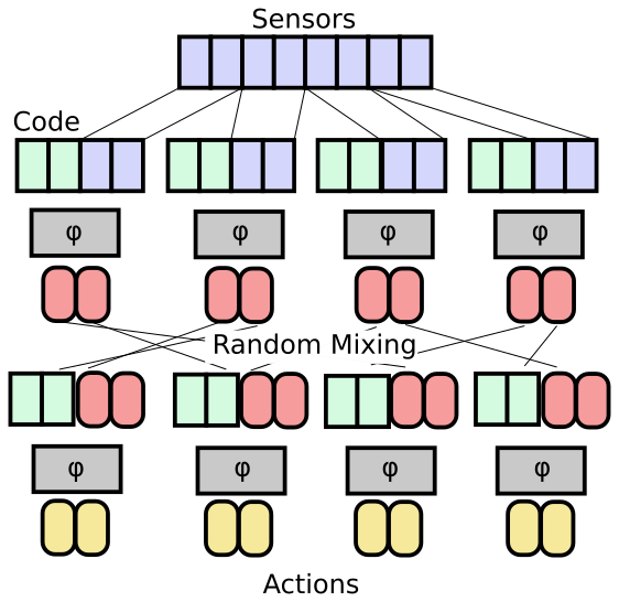
We refer to this variant as ‘mental affordances’ because it chooses the weights Φ to maximize the diversity of attainable policies given the space of codes, rather than maximizing the diversity of physical outcomes. The specific implementation we use works as follows:
- Harvest a distribution of characteristic sensory distributions from the task/environment: {x}
- For each batch, generate a random set of codes {z} (the code space is too large to use a grid as per the original paper).
- Compute all combinations of code and sensory impression over the batch: P x, z = g(x, z, Φ)
- Treating the pattern of actions over sensory impression as a vector for each z, find the distances of each p z vector to the corresponding vector p z′ for z′ ≠ z.
- Via gradient descent, maximize this minimum distance (e.g. set L = – dmin)
For distance we use a clamped L1 norm:  with a =0.25. This prevents the outputs from being driven to their extremal values (which is not a serious problem when the network outputs are probabilities associated with an action, but is more of an issue in the case of continuous control tasks)
A similar loss term may be computed to ensure diversity over sensory inputs given a fixed code (e.g. do the above, but exchange the roles of x and z). This can help when the sensory data isn’t well normalized. However, it may be undesirable in the sense that it tends to suppress policies which ignore the sensor data (which may be the correct solution in some cases). We do not use this term for the experiments presented here.
We additionally regularize the network to prevent the divergence of its gradient and to generally smooth the relationships between nearby codes and sensor inputs. To do this, we compute small random perturbations of the inputs  and
and  , and ask for the L1 distances to be minimized. The size of Φ controls the size of the regularization effect — we generally use 10–³ for the tasks discussed in this post.
Pretraining is done over a period of 1000 gradient descent steps, with 100 codes and 500 sensor impressions used in a single batch. The measurement of the loss does depend somewhat on how many codes/impressions are used (since the minimum distance will get larger the sparser the coverage of the space becomes) — this poses a limitation to using this kind of approach in cases where a single network pass for a code/sensor pair takes a significant amount of memory, and so it would generally be better to pretrain things like convolutional trunks using another method and then using this just to adapt the mapping between high-level features and actions.
Simple control tasks
In investigating simple control tasks, we look at four simple environments provided by AI Gym (https://arxiv.org/abs/1606.01540): CartPole-v0, Acrobot-v1, BipedalWalker-v2, and LunarLander-v2.
We make use of a straightforward dense neural network for Φ, though we use deeper networks than would normally be used for these tasks as we want the code space encoding tasks to be rich enough to contain good solutions to the tasks in question. Specifically, our network is composed of L=16 hidden layers of size H=64 with ReLU activations after each layer. We use d=64 vectors for the task encodings z, and do not use any recurrent scratch space in these cases (as the control tasks we are experimenting with are perfect information).
Therefore, the input of the network is of size N sensors + 64 and the output is of size N actions (with a softmax activation, giving a probability distribution over the possible actions).
We compare two ways of initializing Φ. One is to use random orthogonal initializations (https://arxiv.org/abs/1312.6120) with a gain of √2. The other is to start with random initializations but then train the network to maximize mental affordances.
Subsequent to initialization, we use CMA-ES (specifically https://pypi.org/project/cma/) to optimize the task codes.
Results
You can find the code used to generate the results on GitHub here.
First, let us look at the effects of the affordance pre-training on sensor/action correspondences. We take a set of 500 sensory impressions and 100 random codes from the BipedalWalker-v2 task and plot the first three action components in RGB.
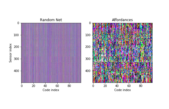
The left panel shows what this looks like for a random network, whereas the right panel shows the case when the network has been pretrained with mental affordances. As a result, the code space addresses a much wider range of sensor-action maps.
Is this enough for the code-space to contain good solutions for the control tasks in question?
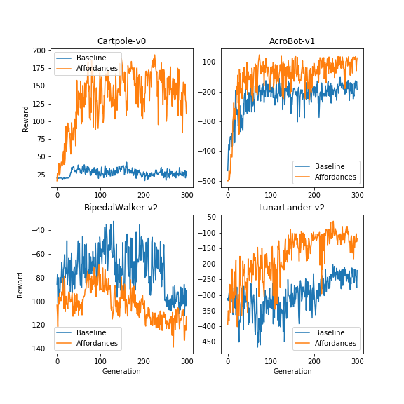
This figure shows the average fitness versus generation for the four control tasks. Except for the BipedalWalker-v2 environment, it is easier for evolution to find better codes in the affordance-initialized network than in the random network. However, even with the affordances the population average performance on each of these tasks is lower than state of the art in all cases.
There is one source of negative bias in this — the population average performance includes the full distribution of new candidate solutions as produced by CMA-ES, and doesn’t necessarily reflect the best solution found. We take these best codes and test them on 10 runs of the corresponding environment with different random seeds, with the following results:
| Environment | Random | Affordances | Leaderboard |
|---|---|---|---|
| Cartpole-v0 | 15 |
120 |
200* |
| Acrobot-v1 | -350 |
-96 |
-42 |
| BipedalWalker-v2 | -5.01 |
-42 |
200* |
| LunarLander-v2 | -270 |
-220 |
300* |
(*: Solved task, where consistently achieving this reward on average counts as solution)
(Leaderboard stats from https://github.com/openai/gym/wiki/Leaderboard)
Here too we see that the ultimate results of this method are still significantly below state of the art and cannot consistently meet the criteria for stably solving these problems.
Discussion
There are three potential explanations for our results, which have relevance to how we should proceed forward with activation-based learning.
- It could be that the O(N) code-space is too small to contain good, tuned solutions, and so there is nothing for evolution to find.
- It could be that while the affordances pre-training improved the situation, it did not do so sufficiently to really cover the space of meaningful sensor-motor contingencies. Alternate methods such as meta-learned initializations (similar to how MAML works), or refinements to the affordances approach, might yet solve this.
- The affordance-trained network does contain good solutions, but our evolutionary approach was insufficient to find them.
Let’s consider these in reverse order. If issue 3 is the case, then using the same affordance-trained network but with different random seeds or learning times for CMA-ES should show a marked difference in the discovered reward. We tried this on BipedalWalker-v2 (which has particularly poor performance) and, even running CMA-ES for 3000 generations rather than 300, we saw no additional improvement. Furthermore, changing the initial standard deviation (to avoid getting caught in local optima of evolution) also appeared to have no effect. So while evolution may be insufficient, that doesn’t appear to be the solitary cause of our problems.
In the case of both issue 2 and issue 1, we would expect to see differences in performance if we retrain the network itself with different random seeds (since then, the network would capture a different subset of the possible sensor-motor contingencies). If the fundamental issue is case 1, then while we should see differences, we shouldn’t see significant improvement even sampling over a number of potential networks Φ since in that case the space of possibilities should be so much larger than our code-space that the approach should amount to random search. On the other hand, if it’s more that the affordance pre-training locks in some early bias but the O(N) codespace is at least in principle sufficient, we’d expect more significant swings with different random seeds.
When we attempted this on BipedalWalker-v2, we saw that some of the pretrained networks had rewards that never became better than -100 on average, while others achieved scores around -40. So it does seem like we’re seeing behaviors that have a fairly high chance of either being included or excluded based on the random seed (e.g. closer to 50/50 than 1/99).
Another test we can do is to shrink the code-space and see if the solutions get worse. If the issue is the pre-training then we wouldn’t necessarily expect that shrinking the code-space will prevent us from finding comparable solutions in the case of more complex tasks like the walker. We find in fact that using a code-space of dimension 3 produces comparable (or even better) results than a code-space of dimension 64 on the BipedalWalker-v2 task.
So the evidence appears to favor what we call issue 2 — that not just any network Φ will give us a good repertoire of sensor-motor contingencies, and that the way we initialize or pretrain Φ is likely to dominate whether we can eventually find performant codes for a given distribution of tasks.
Next steps
Testing Issue 1 vs Issue 2
Is there some other way we can check if the code-space is big enough, so we could exclude case 1? Well, there’s a lot of evidence that the full O(N²) dimensional space of the weight matrices isn’t needed either to represent solutions, or even to learn them. Things such as Weight Agnostic Neural Networks (https://weightagnostic.github.io/) show that the actual floating point values of weights is less important than their topology. Results elsewhere show that large weight matrices are beneficial for learning, but once the network has been trained it can often be distilled down to a much smaller network that is equally performant (https://arxiv.org/abs/1503.02531).
One check we can consider is something akin to matrix factorization. We can in principle write the N × N weight matrix W as the product of a N × B matrix and a B × N matrix. This reduces the number of available parameters from N² to 2NB, while maintaining the structure of the architecture. If we examine how this impacts performance, we can see whether the parameterization capacity is really the problem.
General ideas about code space expressivity
Moving forward especially as it relates to Badger, we would like to know if it is possible to determine how expressive different code-spaces are. Will activation-based encoding of the entirety of the task-specific parts of the behavior always struggle against capacity limitations, or would breaking the task-coding up across a population of experts actually help?
Let’s consider that the problem is really what we called ‘issue 2’ — that finding a single network Φ whose inputs parameterize all potential sensor-motor contingencies that we might want to express is difficult. Why might the affordance-based initialization fail to provide this?
When we maximize the minimum distance between sensor-motor contingency vectors (actions mapped to sensor impressions), we assume that what we get will asymptotically favor a uniform covering of the space. However, if we consider what happens when vector spaces become high dimensional, there’s a phenomenon where Gaussian random vectors become concentrated on the surface of a hypersphere in that space, and pairs of randomly chosen vectors are highly likely to be nearly orthogonal to each-other. So our sense of ‘covering’ a space by evenly spacing things out may be harder and harder to detect as the vector spaces become large.
In that case, breaking things up into modular subspaces of lower dimension should help us better determine if we are spanning the space of possibilities uniformly, even with reasonable batch sizes. The idea here would be that, if we have Ns sensors, No outputs, and a desired code space of size Nc, then rather than training one network that takes sensors + code to outputs, we chunk up the sensor space, output space, and code space into blocks of dimension 3 or 4, each of which having its own network Φ pre-trained using affordances.
Conclusions
When we move from a universal learning method such as gradient descent on neural networks (which are known to be able to represent any function) to learned learning methods, learned ways of representing policies and tasks, etc, then we risk losing that universality property — an agent which is trained to learn may no longer be able to learn arbitrary things.
Here, we investigated whether using vector codes for tasks as inputs to a randomly initialized policy network would be sufficiently expressive to capture solutions to unseen tasks, even using subsequent optimization over the vector codes. We found that this was not the case, and that policies became highly concentrated when using a random policy network. In other words, most behaviors are hard or impossible to express.
By pretraining the policy network in an unsupervised manner, we could request the set of input-output maps represented by the space of task codes to be as diverse as possible. In this case, we did find solutions or near-solutions to many tasks, but even here sometimes (randomly, from trial to trial) the solutions were or were not included in the space spanned by the policy network. We conclude this is not because the task codes have too low of a capacity to represent the solutions, but that even when asking for a high diversity set of policies, we lack any kind of guarantee of coverage — every time we train it, we get random blind spots.
This suggests a solution: by breaking down the policy networks into smaller pieces, we should be better able to guarantee coverage of the space of policies in each sub-network. These can then be composed together in a similar fashion to cover larger spaces through combinatoric explosion. Our next steps will involve studying this concept of expressivity as it relates to modular architectures and different ways of representing policies or programs in learned systems.
Acknowledgments
A lot of these ideas crystalized out of the biweekly Belief Empowerment research meetings held in Tokyo over the last six months, which covered things such as how intrinsic motivations like empowerment could be applied to purely mental states. In particular, we would like to thank Martin Biehl, Lana Sinapayen, Nathaniel Virgo, and Olaf Witkowski for extensive feedback with respect to the general idea of ‘mental affordances’, and to the specifics of how it is used here.


