The thirty-fourth conference on Neural Information Processing Systems took place last week. Unlike last year where many of us traveled to Vancouver in person, this year GoodAI, just like everyone else could only attend virtually. With nearly 2000 research articles and countless workshops and tutorials there was an overwhelming amount of exciting new ideas, fascinating research, deep discussions and virtual socializing done in the seven days over which the conference spanned.
In this post we outline some of the highlights of the conference, in particular from the point of view of research that in one form or another either relates to research on our Badger architecture or is relevant to our present endeavours. This is only a snippet of some of the relevant work that was presented at NeurIPS, and by no means is exhaustive. If you are also excited about any of the topics mentioned below, have experience in the related field or you believe you could contribute to it and would like to discuss with any of our team members, please contact us at info@goodai.com.
Most related topics
- Continual learning
- Meta-learning
- Open-endedness
- Modular (meta-)learning
- Optimization in modular systems
- Meta-learning of lifelong learning
- Self-referential learning
- Learned optimizers
- Multi-agent reinforcement learning
- Graph neural networks
- Learned communications
Most related methods
The following list of methods are very closely related to our Badger architecture. It is exciting to see other research groups attempting to pave way for and approaching the building of more general decision making system that are based on modularity, meta-learning and learned learning algorithms. Method [1] is described in more detail below.
- Meta-Learning Backpropagation And Improving It. Louis Kirsch, Jürgen Schmidhuber. [paper] [supplementary] [poster]
- MPLP: Learning a Message Passing Learning Protocol. Ettore Randazzo, Eyvind Niklasson, Alexander Mordvintsev. [paper] [supplementary] [poster]
- Learning not to learn: Nature versus nurture in silico. Robert T Lange, Henning Sprekeler. [paper] [poster]
- Training more effective learned optimizers. Luke Metz, Niru Maheswaranathan, Ruoxi Sun, Daniel Freeman, Ben Poole, Jascha Sohl-Dickstein. [paper] [poster]
- Related workshops
- Related tutorials
1. Meta-learning backpropagation and improving it: General Meta Learning and Variable Sharing
The 2020 workshop on meta-learning hosted a talk on General Meta Learning. The work, described also in a paper accepted by the workshop by Kirsch and Schmidhuber, tackles meta-learning learned learning rules that generalize. There are several similarities with the Badger architecture.
Motivation and context
There are two main approaches to meta-learning. The first one is based on changing (fast) weights in the inner loop, which itself is evolved over extended periods of time in an outer loop (fast and slow weights). The other approach is based on changing RNN activations.
The first approach usually introduces new mechanisms and complexity into the architecture. The second approach, on the other hand, has limited generalization capability with respect to the total parameter count, since the number of inner-loop parameters (RNN activations) is much smaller than number of outer-loop parameters (weights).
The presented work addresses the two issues by implementing general activation-based meta-learning (thus avoiding new complexity), and introducing shared parameters to improve the generalization capability of the learned algorithm.
Model description
The Variable Shared Meta RNN, a.k.a. VS-Meta RNN, is composed of multiple small RNNs (LSTMs in fact) that are placed in a 2D grid of size $A \times B$. RNNs in this grid can communicate over connections of a fixed sparse topology. Communication is facilitated by the interaction matrix $C$ with learned shared parameters.
The model has the ability to implement meta-learning in activations. Since the parameters of VS-Meta RNNs (as well as the interaction matrix) are shared, it avoids the main problem of this type of meta-learning architectures (where the number of inner-loop parameters is smaller than the outer-loop parameters, which causes lack of generalization abilities).
The model is very flexible, since part of the RNN state can be interpreted (used) as a “neuron activation” and another part as a “weight”. The ability to implement multiplicative interactions (between states and weights) are included in the LSTM gating mechanism.
Model interpretation
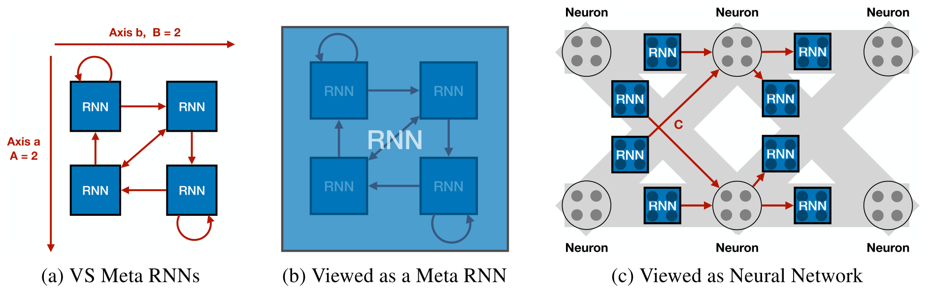
There are multiple interpretations of the VS-Meta RNN. The first sub-image (a) in the figure above (from Kirsch & Schmidhuber) shows the basic structure of the method. The model can be viewed as a single Meta-RNN where some entries are shared or zero (b). Lastly (c), the VS-Meta RNN can be seen as implementing a neural network where outer-loop learned parameters determine the nature of weights and biases: how these are used in the forward computation and the learning algorithm by which those are updated. Here, neurons correspond to intermediate computation results of the interaction term which are fed back into the RNNs.
Experiments
The algorithm learned via the VS-Meta RNN approach should have the ability to implement backpropagation. There were two types of training setups that test this.
- In the “backprop-cloning” setting, the VS-Meta RNN is explicitly trained to store the $w$ and $b$ in the RNN activations, to compute the forward pass of the neural network $y = tanh(x)w + b$ and then to update the $w$ and $b$ according to the backpropagation algorithm.
- In the harder-to-train “meta-learning from scratch” setting, supervised signal to the inner parts of the network is not provided anymore. Rather, meta-learning is done from the input data and the error signal only. The CMA-ES is used for optimizing the weights in this case.
Meta-training is done either on random data or on the MNIST dataset. Generalization of the learned algorithm is then evaluated on MNIST or Fashion MNIST.
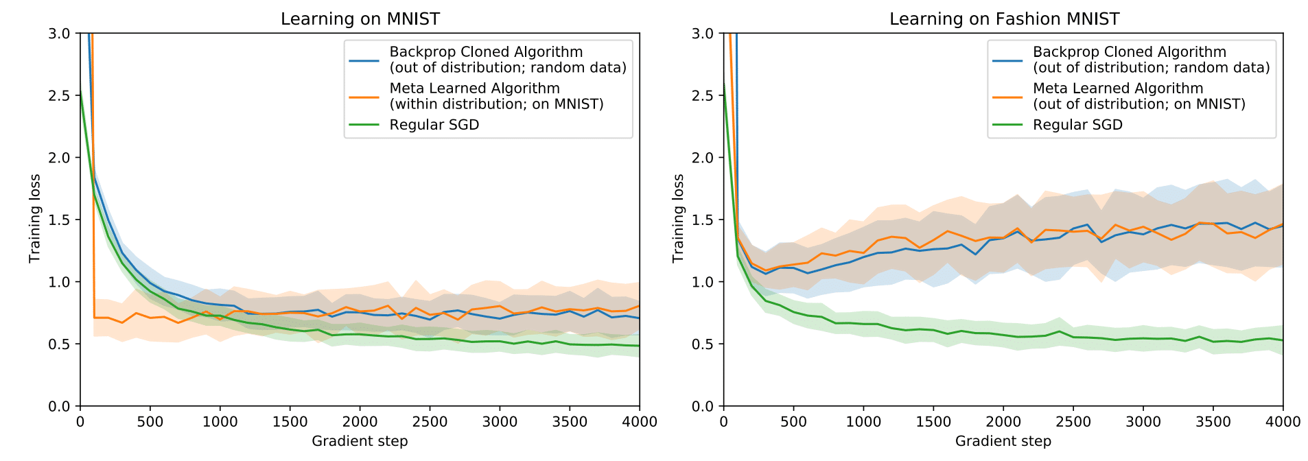
The above plots (from Kirsch & Schmidhuber) show the meta-testing loss of VS-Meta RNN that was optimized to implement backpropagation in its recurrent dynamics on random data (blue) or on MNIST (orange). Here, the learning is done purely by unrolling the LSTM. The left plot shows meta-testing on MNIST, while the plot on the right shows meta-testing on Fashion MNIST.
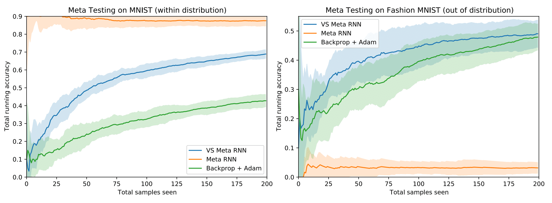
The second experiment (plot from Kirsch & Schmidhuber) tests the ability to learn a supervised online learning algorithm from scratch. Here, the VS-Meta RNN is meta-trained on MNIST to minimize the sum of cross-entropies over 200 data points starting from random initializations of hidden states. During meta-testing on MNIST/Fashion MNIST (the figure above) the authors plot the total accuracy computed on all previous inputs on the y axis. We can see that the VS-Meta RNN learns faster than online Backprop+Adam baseline and generalizes to out-of-distribution data (Fashion MNIST) well, while a standard Meta-RNN overfits to the in-distribution data (MNIST).
It has been shown that the VS-Meta RNN is able to learn a learning algorithm in the activations from scratch. Compared to a standard Meta-RNN, simply by incorporating the shared parameters and sparse connectivity, the VS-Meta RNN is able to learn quickly and the learned learning algorithms generalize to out-of-distribution data.
Relation to Badger
We see tight connections to the Badger architecture.
- The reuse of RNN modules, which can be seen as corresponding to Badger experts.
- The training by backpropagating through unrolled RNN progress.
- The sharing of parameters to allow scaling and generalization. We are excited to see research so close and relevant to our own efforts!
2. Backpropagation-free learning: CLAPP
There has been recent interest in exploring methods that no longer rely on backpropagation. This has been reflected in this year’s conference with the beyond backpropagation workshop and papers such as GAIT-Prop, CLAPP, ZORB and Brain-prop. Works such as CLAPP and Brain-prop have commonalities in their decisions to account for the plasticity of neurons while training.
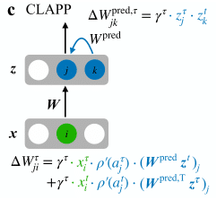
The CLAPP paper is an unsupervised learning rule that takes inspiration from Greedy Infomax from Putting an End to End to End, and Contrastive Predictive Coding methods. The result is the Contrastive Local And Predictive Plasticity approach, which is a loss method that uses positive and negative samples in a hinge-like additive loss.

The learning rule using this loss is gradient free, and makes use of recurrent predictive connections $W^{\text{pred}}$, the pre- and post-synaptic values $i, j$, and a global plasticity value $\gamma^{\tau}$ to compute updates to $W$.
The authors have found that the CLAPP method is performant on the STL-10 and LibriSpeech datasets, outperforming supervised SGD on STL-10:
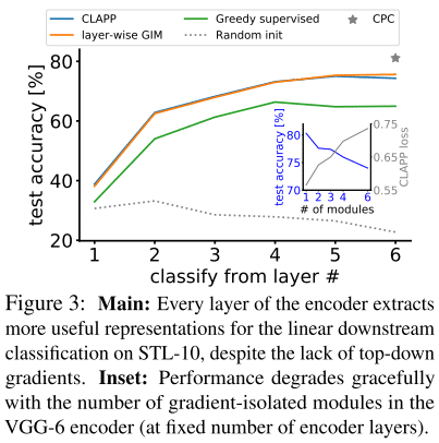
All above figures are from (Grill et al. 2020).
Relation to Badger
CLAPP is just one exciting paper that deals with local learning rules at this year’s NeurIPS. We are interested in these biologically plausible methods, not because biological plausibility is a requirement for Badger, but because the mechanisms that they require lead to useful attributes. Local updates enable more parallel training, and the plasticity of neurons can alleviate forgetting in continual learning settings. We are excited to follow this thread of research and its implications for the future of the Badger architecture.
3. Learned update rules: paper highlights
NeurIPS 2020 featured several exciting examples of recent work in the area of learned update rules. Here, we will first highlight Meta-learning through Hebbian plasticity in random networks (Najarro and Risi 2020), then briefly discuss a few other very interesting works that also address the learning of Hebbian update rules.
Meta-learning Hebbian plasticity
In Meta-learning through Hebbian plasticity in random networks (Najarro and Risi 2020) the authors train agents by optimizing Hebbian plasticity parameters instead of fixed weights. Agents are randomly initialized and must adapt their weights during their lifetimes using a Hebbian ABCD rule:
$$ \Delta w_{ij} = \eta_w(A_w o_i o_j + B_w o_i + C_w o_j + D_w) $$
The architecture, trained using evolution strategies, was tested in a car racing 2D environment and on a MuJoCo-like 3D locomotion task. The results were encouraging. In the locomotion task, the Hebbian agent had some success in adapting to a new morphology not seen during training. A baseline agent with fixed weights failed at this. In addition, the Hebbian agent proved resilient to weight perturbations, recovering quickly after a large part of the weights had been zeroed out.
The model presented in the paper learns different parameters and learning rate $(A,B,C,D,\eta)_w$ for each synapse. What happens if you reduce the number of parameters, sharing them between synapses? The authors told us that they have found that extensive parameter sharing is possible while maintaining good results on the tasks. More systematic investigation is needed to understand the effects of parameter sharing in this setting. We are looking forward to learning more about this.
The authors have made their code available at https://github.com/enajx/HebbianMetaLearning.
Discovering synaptic rules from observational data
A meta-learning approach to (re)discover plasticity rules that carve a desired function into a neural network (Confavreux et al. 2020) explores the possibility of discovering synaptic update rules from data describing neural and synaptic behavior. In proof-of-principle experiments, the authors succeeded in recovering Oja’s rule and a related Hebbian rule as well as a known update rule for spiking neurons. Next, they plan to apply their method to data from biological neurons.
Hebbian memory
In H-Mem: Harnessing synaptic plasticity with Hebbian Memory Networks (Limbacher and Legenstein 2020) the authors use Hebbian learning to implement associative memory. This is an interesting approach to adding medium- and long-term memory to an agent. The model is capable of one-shot memorization of associations between stimulus pairs and also performs well on the bAbI question answering data set.
Improved Hebbian learning
Finally, HebbNet: A Simplified Hebbian Learning Framework to do Biologically Plausible Learning (poster at the Beyond Backpropagation workshop) proposes simple modifications to Hebbian learning that produce dramatically improved results. An important trick is sparse updates in the outer loop: instead of adjusting the plasticity everywhere, update only the one percent of the parameters for which the magnitude of the gradient is the largest.
Relation to Badger
There are numerous potential advantages to replacing end-to-end backpropagation with local learning rules. Among them are the ability to learn without a gradient, easy parallelization, and the possibility of scaling up a system with little or no retraining, all properties we aim for in Badger. In the real world, one often has to learn from a few examples only and sometimes even, a mistake is not an option. In such cases, one needs to rely on more efficient (and more prior-laden) learning rules than the very broad and general backpropagation update rule.
4. Representation learning: BYOL and SurVAE Flows
Two new techniques for learning latent representations were presented at the conference, which may see a wide adoption in the coming years and change the way we do ML. Those two techniques are BYOL, or Bootstrap your Own Latent (Grill et al. 2020) , and SurVAE Flows (Nielsen et al. 2020). Below is an explanation for why those two techniques overcome existing limitations and thus why they may gain widespread adoption and are relevant for our research.
BYOL
Problem setting
BYOL may be the next step for contrastive learning. Since it regained interest in 2018, contrastive learning has taken over as the unsupervised learning method of choice, especially in the form of SimCLR (Chen et al. 2020), which was the baseline that everyone was trying to beat at NeurIPS 2020. The problem with contrastive learning is that you need negative examples. E.g. for each image (let’s say we have an image dataset), you need examples of images which are not in the same category. Needing negative samples is in fact three problems. From simplest to most complicated, those are:
- It’s another annoying technical complication.
- The training works better if the negative examples are difficult negative examples, that is, negative examples which look like the positive example but are not (the bird which has the same background as the airplane but is not a plane, the truck as a negative example to a car, etc.), but that is not an easy thing to do in practice, and what is an easy or hard negative example changes as the training progresses.
- It can be shown (Song and Ermon 2020) that contrastive predictive coding is a lower bound on the mutual information between the latent representation of the image and the image itself. But the problem is that it is upper-bounded by $\log(m)$ where $m$ is the number of negative examples (and so ideally one would need an infinite amount of negative examples). That means that if you want to have a lot of information in the latent representation, one needs a lot of negative examples for each positive example. For example, in ImageNet, where there are thousands of possible categories, one needs thousands of negative examples for each positive example. This is not feasible in practice. So the theory tells us that with a finite number of negative examples, the quality of the representation obtained with contrastive learning will always be limited.
Method
Basically, BYOL is the Mean Teacher (Tarvainen and Valpola 2017), a semi-supervised technique, without the supervised learning signal. It proceeds as follows:
- Take the input image and apply two different “noises” to it that shouldn’t change the label (different crops, rotations, change of colours, etc.).
- Pass one of the images to the teacher network which will provide the target (and not have its weights modified through backpropagation) and the other to the student network (which has the same architecture as the teacher network).
- The student network is learning through backpropagation to achieve the target latent vector given by the teacher network. This encourages latent representations which are invariant to the different noise sources applied to the input.
The question of “how are teacher network weights set” is yet to be answered. Like in Mean Teacher, the network is randomly initialized and the teacher is simply an exponential moving average of the student network.
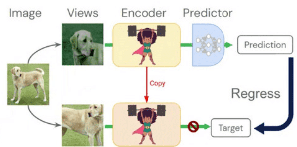
An overview of the approach can be seen in the figure above (from the conference presentation)
Results
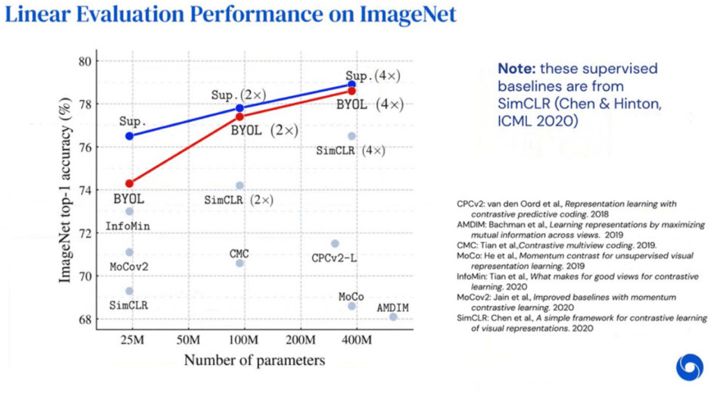
BYOL (red line) is almost reaching the accuracy of supervised learning (blue line) on ImageNet. This is very impressive. (Figure from the presentation).
SurVAE Flows
The goal of SurVAE Flows (Nielsen et al. 2020) is to one-up all of GANs, Variational Autoencoders (VAEs), and Normalizing Flows and be your one-pit stop solution replacing the three different solutions you needed before.
Problem setting
Each of GANs, VAEs, and Normalizing Flows have their pros and cons. Here is a little summary table of them:
| Can sample data | Can encode data to latent | Provides high quality samples/reconstructions | Latent and data sample can have different dimensions | Easy to train | |
|---|---|---|---|---|---|
| GANs | ✔️ | ❌ | ✔️ | ✔️ | ❌ |
| VAEs | ✔️ | ✔️ | ❌ | ✔️ | ✔️ |
| Flows | ✔️ | ✔️ | ✔️ | ❌ | ✔️ |
The problem with GANs is that if one starts from a sample image, there is no way to obtain its latent code $z$ because there is no encoder. GANs are also harder to train, though this problem is getting gradually less severe. On the flip side, GANs provide the best quality samples subjectively, for instance generated human faces can already look photo-realistic. The problem with VAEs is that they provide comparatively low quality (“blurry”) samples. The major problem with Normalizing Flows, which have exploded in popularity in the last two years or so, is that the dimensionality of the input has to be the same as the dimensionality of the output, so if one has a high resolution image, one has to encode it in a latent code of the same dimensionality.
Method
Every layer in a Normalizing Flow is a bijection. SurVAEs generalize flow to allow for surjections either in the encoder (which is the scenario which makes sense if you want your latent code to be a compression of your data) or the decoder but still otherwise preserves the structure of the Normalizing Flow. Furthermore, the authors put SurVAE Flows inside a theoretical framework which includes both VAEs and Normalizing Flows.
Results
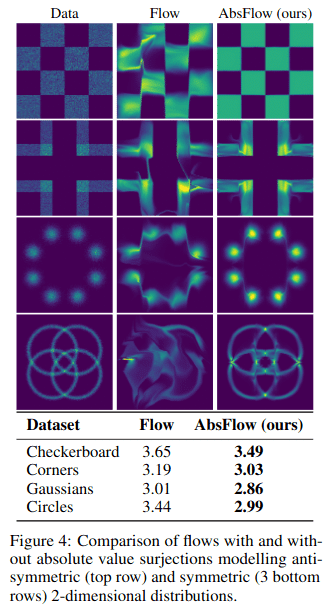
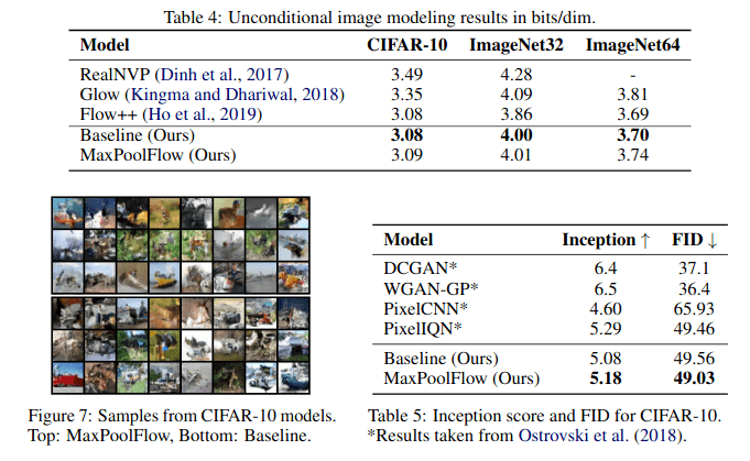
The results listed above (from Nielsen et al. 2020) should be interpreted as proof-of-concept experiments showing the capabilities of the SurVAE Flows. At the moment, they don’t reach the power of GANs or WaveNet-style networks, although they can get close in some benchmarks. Note that the bolding in the results above is used to show the better of the authors’ methods, not the best of all methods.
Relation to Badger
Ideally we would want a Badger agent to be able to deal with environments which don’t necessarily provide an explicit reward function, or which doesn’t come with labeled data. How to properly do unsupervised learning is a question of importance for Badger. Both BYOL and SurVAE Flows are promising new directions in unsupervised learning.
5. Deep implicit layers
Implicit layers offer an interesting way how to formulate the learning process of
a neural network. Instead of common explicit layers in the form $y = f(x)$
an implicit form $g(x,y) = 0$ is used. There was a tutorial on this exciting topic at the conference.
Implicit form has several advantages:
- Powerful representations: compactly represent complex operations such as
solving optimization problems, integrating ODEs, etc - Memory efficiency: no need to backpropagate through intermediate components,
via implicit function theorem
Deep Equilibrium Models
Deep Equilibrium Models (DEQ) (Bai, Kolter and Koltun 2019) represent modern deep networks using a single implicit layer while having near SOTA performance in large scale NLP and vision tasks.
Traditional deep networks applied to an input $x$ can be described as $z_{i+1} = \sigma(W_iz_i + b_i)$.
With the introduction of two constraints:
- fixed input – input is constant during computation of NN result
- shared weights – weights of all layers are the same
we can simplify to $z_{i+1} = \sigma(Wz_i + x)$ and apply the same function repeatedly to the hidden units. In many situations the network can be designed in such a way that it will converge to some fixed point or equilibrium point: $z^* = \sigma(Wz^* + x)$. Such model is a minimal DEQ.
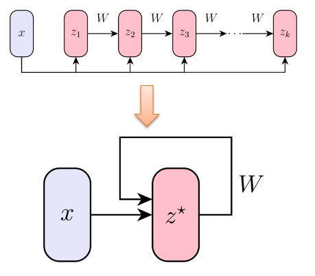
This procedure can be seen in the above figure (from a tutorial on this topic).
Training of DEQs
Forward pass:
- Given $(x,y)$, compute equilibrium point $z^* = f(z^*, x, \theta)$
- Compute loss $L(z^*, y)$
Backward pass:
- Compute gradients using implicit function theorem: $\partial L(\theta) = \partial_{z^*}L(z^*, y) * T$ where $T$ is a term that can be computed directly from an automatic differentiation system and $z^*$ (detailed description) without the need of backpropagating through optimization in the forward pass.
Benefits
- Computational graph for backpropagation is reduced significantly. Instead of backpropagating through all layers or iterations of the inner-loop, using a mathematical trick we can compute the gradient just from an equilibrium point and the VJP (vector Jacobian product) computed by an automatic differentiation system.
- Workload is transfered from inner-loop inference to computation of the equilibrium point where a sophisticated optimizer can be used, e.g. Anderson Acceleration.
- Expressing a whole NN as an implicit layer brings interesting capabilities as presented in Multiscale Deep Equilibrium Models (Bai et al. 2020) – Effective simultaneous learning of image classification and semantic segmentation. CNNs for different scales coexist side by side and are driven to equilibrium simultaneously.
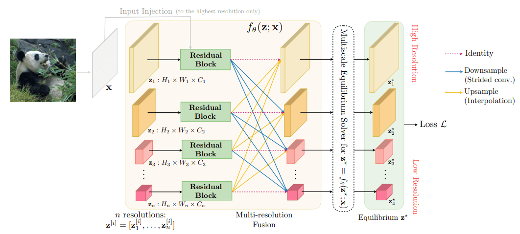
The above figure is from (Bai et al. 2020).
Relation to Badger
One of the key focal points of Badger architecture is finding an expert policy that can sustain learning over long horizons. In the traditional viewpoint, this requires backpropagating through very long inner loop rollouts. The work on DEQ is intriguing through its potential for significantly reducing lengths of inner loop rollouts and thus speeding up learning, or in some cases even enabling it.
6. Designing Learning Dynamics (Tutorial)
Marta Garnelo, David Balduzzi and Wojciech Czarnecki presented an overview of different principles and methods that can be used to design learning dynamics that take into account how populations of agents interact. The tutorial is divided in three different sections that explain how to design interactions between agents that produce different learning dynamics. Although the tutorial does not dive deep into technical details, it introduces the core principles and methodologies needed to understand learning from an evolutionary game theory perspective.
The dynamics of learning objectives
The first part of the tutorial focuses on showing the difference between optimization and evolution. It explains the differences between how optimization or learning algorithms behave in isolation vs how they behave when they interact with a population of agents and their environment. After a gentle introduction to game theory, it explains the main building block used to design learning dynamics for populations of agents: Pairwise interactions in zero-sum games.
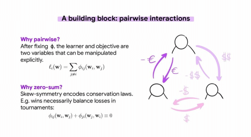
The above figure is from the tutorial presentation.
A single zero-sum interaction between two players implicitly encodes a function space of objectives that allow to evaluate players in a game relative to each other instead of relying on a global fitness function. By defining a player as a basic unit of abstraction and optimizing populations instead of individuals, the objectives become population-dependent.
The dynamics of artificial evolution
This part of the tutorial is about how to design learning dynamics in evolutionary algorithms, and how these can be used to optimize populations. It explains how to use zero-sum interactions can be used to evolve a population in a multi-task setting using partial ordering and MAP-Elite, and how different dynamics can produce different agent behaviors depending on the structure of the game that is being learned. Those principles do not only allow for a lot of flexibility and scale naturally to n-agents, but they also apply when the underlying function to be optimized is unknown.
Then, the tutorial goes one step further and explains how it is possible to measure the performance of an agent with respect to the entire population in the context of ensemble models. This approach allows to easily express diversity preservation methods, and training entire populations can lead to more open ended learning regimes. Finally, this part presents an example of multi-level evolution with two phases: an outer loop that defines rewards for a given agent, so it performs well in the population, and an inner loop that optimized the reward defined by the outer loop.
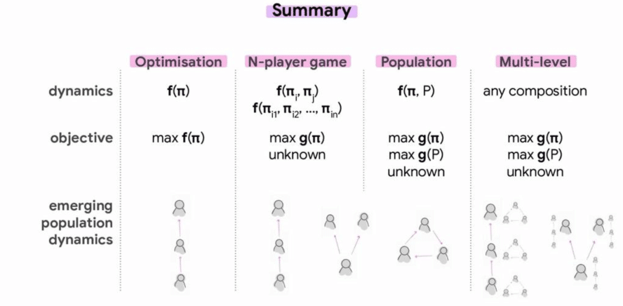
The above figure is from the tutorial presentation.
The dynamics of training populations
The last part of the tutorial is focused on how to rate agents when there is no absolute measure of performance. It first explains different techniques for rating agents such as ELO rating and its extensions, and how their principles can be applied to rating populations of agents by measuring relative population performance and effective diversity.
Finally, the tutorial covers different methods for choosing opponents in a population-based training setting like Policy Space Response Oracles (PSRO) and some other variants. The basic design principles for population-based training are shown, and the effect that the different interaction dynamics have on the performance and diversity of a trained population of agents is demonstrated.
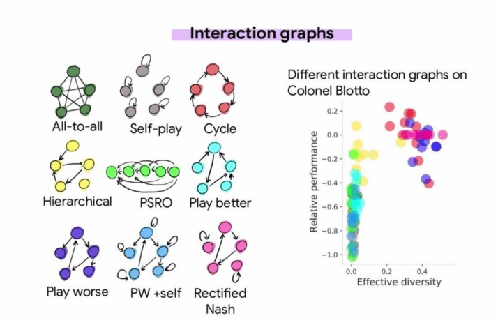
The above figure is from the tutorial presentation.
Relation to Badger
We see a direct connection between the topics presented in the tutorial and design considerations for Badger architecture, which is a network of policy-sharing modules that need to adapt to a dynamically changing environment.
References
- Oord, A.V.D., Li, Y. and Vinyals, O., (2018). Representation learning with contrastive predictive coding. arXiv preprint arXiv:1807.03748.
- Chen, T. at al., (2020), A Simple Framework for Contrastive Learning of Visual Representations. ICML 2020.
- Song, J. and Ermon, S., (2020), Multi-label Contrastive Predictive Coding. NeurIPS 2020.
- Grill J-B. et al., (2020), Bootstrap your own latent: A new approach to self-supervised Learning. NeurIPS 2020.
- Tarvainen, A. and Valpola, H., (2017), Mean teachers are better role models:
Weight-averaged consistency targets improve
semi-supervised deep learning results. NeurIPS 2017. - Nielsen, D. et al., (2020), SurVAE Flows: Surjections to Bridge the Gap between VAEs and Flows. NeurIPS 2020.
- Najarro, E. and Risi, S. (2020), Meta-learning through Hebbian plasticity in random networks. NeurIPS 2020.
- Confavreux, B., et al., (2020), A meta-learning approach to (re)discover plasticity rules that carve a desired function into a neural network. NeurIPS 2020.
- Limbacher, T. and Legenstein R., (2020), H-Mem: Harnessing synaptic plasticity with Hebbian Memory Networks, NeurIPS 2020.
- Bai, S. and Kolter, Z. and Koltun, V. Deep Equilibrium Models. NeurIPS 2019.
- Bai, S. and Kolter, Z. and Koltun, V. Multiscale Deep Equilibrium Models. NeurIPS 2020.
- Walker, H.F. and Ni, P., (2010), Anderson Acceleration For Fixed-point Iterations, Walker, Ni, 2011, SIAM J. Number. Anal., Vol. 49, No. 4, pp. 1715-1735
Authors
Jaroslav Vítků, Isabeau Prémont-Schwarz, Simon Andersson, Petr Hlubuček, Guillem Duran Ballester, Joseph Davidson, Martin Poliak, Jan Feyereisl


![[poster]](https://meta-learn.github.io/2020/papers/34_poster.png)
![[poster]](https://meta-learn.github.io/2020/papers/7_poster.png)
![[poster]](https://meta-learn.github.io/2020/papers/33_poster.png)
![[poster]](https://meta-learn.github.io/2020/papers/54_poster.png)