Trainability of Badger – Why is Badger so hard to train?

By Petr Šimánek
GoodAI
FIT CVUT

Summary

• Badger
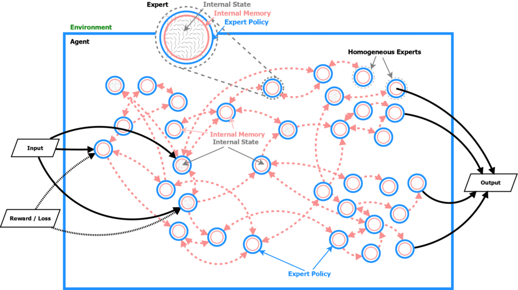
  • An agent is made up of many homogeneous experts.
  • All experts share the same expert policy but have different internal memory states.
  • The trained expert policy is able to adapt to and solve a range of different and novel tasks (long-term goal).
• We study a special case of Badger called Micro-Badger applied to a toy task called Guessing Game.
• Symmetries in Badger and the learning plateaus are investigated. Reasons for the plateaus are similar to reinforcement learning and are caused mostly by symmetries.
• Micro-badger follows a similar learning strategy to meta-learning and reinforcement learning models. This is investigated by the frequency principle.
• Mutual information between the experts shows that experts need to learn how to be more diverse to initiate learning.
• Binding information reveals a growing organization of the experts in micro-badger during the training.
• Next steps:
  • Apply architecture changes that allow to divide a composite task to single tasks and solve it without competing gradients or meta-learning to find a better loss function.
  • Apply optimization methods that allow “saddle escaping”.
  • Explore the effects of different topologies (weakly or strongly connected) and the effect of different eigenvalues of the Laplacian.

Introduction

Badger [Rosa] is a multi-agent meta-learning architecture with homogenous agents called experts. It turns out that Badger is usually quite hard to train. We mostly observe multiple plateaus during the training and it generally takes many thousands of iterations to converge. 

To understand why Badger is hard to train, we need to understand first how Badger learns, using a toy task. We try to understand the plateaus, what happens during this period, and why the plateaus are there in the first place. We explore if Badger prefers to solve low frequencies first (like DNN) or if it solves all the frequencies at the same time; the bias towards lower frequencies is called F-principle [Zhi-Qin]. Mutual information between experts during the inner loop and the outer loop is investigated to understand what happens during the plateaus and what is necessary to escape the plateaus. Further analysis based on Binding Information shows that the self-organization of experts keeps growing during the training.

We want to understand if Badger behaves like RL and meta-learning and to suggest some ways to improve the learning.

Badger

Badger is a general meta multi-agent learning framework with homogenous expert policy. It usually works in the outer/inner loop setting. The outer loop is currently used to learn the policy that the inner loop experts will follow to solve the task. The current inner loop policy is trained only for a specific task. In the future iterations of Badger we aim for a more powerful inner loop that is able to learn to solve a range of different tasks.

Micro-Badger

Micro-Badger is one of the existing implementations of Badger with some specific features. The outer loop learns the weights of a recurrent neural network. Each expert in the inner loop is a recurrent neural network with the same weights. The topology of connections between the experts is created randomly. Each expert will send its output to some other experts and will receive outputs of other experts as well. This happens only in micro-badger, Badger’s long term goal is to discover the policy inside the inner loop. 

Guessing Game

We want Badger to solve a task called guessing game. Think of a number and let the experts guess it, using the difference from the correct answer as feedback on the guess. Think of N numbers and let the experts guess them. The experts in the inner loop must communicate and try to guess the numbers. The outer loop in the Badger tries to train the experts so that they can solve the problem. The only feedback the experts receive, even for the case with N numbers, is a single scalar – the mean squared error of the guess.

Symmetry

We will talk about symmetry repeatedly, it is important to explain what we mean by symmetry:

Definition 1. Symmetry: Any object which displays some kind of repeating pattern in its structure is said to be symmetric [Barakova]. 

There are many symmetries in the system, e.g.:

1. The symmetry between the neurons in neural networks.
2. The sign symmetry of the sigmoid function in the gate in RNN.
3. The symmetry between the experts in micro-badger – at the beginning of the training, the experts are interchangeable.
4. The symmetry of the Guessing Game, reducing error in the first dimension makes the same overall effect on loss as reducing the error in the second dimension, etc.
5. The symmetry in the weights (this symmetry is only reduced by random initialization [Barakova]).

The initial symmetry between the experts and in the RNN (together it is symmetry in the architecture) and initialization by small values allows the algorithm to choose a path in any direction while reaching similar local minima. 

The learning process starts in the area situated symmetrically between the different learning subspaces (symmetrical). During the initial training phase, the guidance from the learning algorithm tries to break the symmetrical state of the network and to force the remaining search in one of the possible subspaces. The bearer of this initial symmetry is the highly parallel (symmetrical) architecture and the choice of the initial state. In the case of the guessing game, it means to choose the dimension Badger tries to solve first. 

Plateaus in training

There are usually multiple plateaus during training for the guessing game task. These are connected to the symmetries in the system [e.g. Barakova]. The gradient method cannot decide between multiple similar options and is therefore indecisive.  

In our case by symmetries, we mean that there is permutation symmetry between the experts and symmetry in the guessing game. Usually, there is one plateau at the beginning where Badger predicts only zeros. After a while, it does predict different numbers than zeros (all the same though), and then it learns to guess the numbers one by one. During each of the plateaus, the gradients are very small, and the Hurst exponents are very close to 0.5 – it means that there is no autocorrelation (no anticorrelation either) – no long term behavior, the error changes randomly. Badger moves randomly around the plateau/saddle until it escapes it.

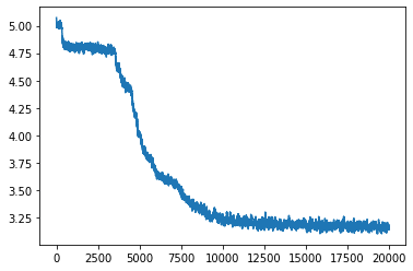
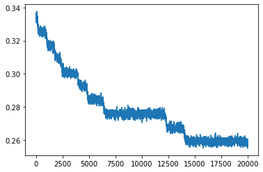The error of the guessing game, N=20

The very last plateau is the converged solution. We computed the Lyapunov exponent of this section (using nolds library https://pypi.org/project/nolds/) and the largest exponent is positive, which suggests that the solution is not asymptotically stable. It means that there is no guarantee that the solution will stay close to the minimum.

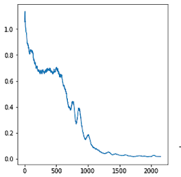The error of the guessing game, N=3, Converged solution since 1500th iteration.

Why are the plateaus present? 

There are four explanations and they are neither competing nor exclusive:

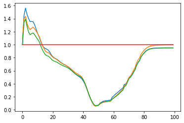
1. One reason is described in [Schaul], they call it ray interference. Ray interference often occurs in reinforcement learning, where the objective function can be decomposed into multiple components. In the guessing game, the loss is MSE – mean of individual errors in each dimension. In the following images, the initial values are close to zero and the error is minimized by moving to [1,1]. We see that supervised learning usually chooses a very straightforward trajectory to minimize the error. RL, on the other hand, solves the dimensions one by one – first moving to [1,0] or [0,1] and only after that to [1,1]. The same applies to Badger, Badger tries to reduce error by canceling error in one dimension at a time.

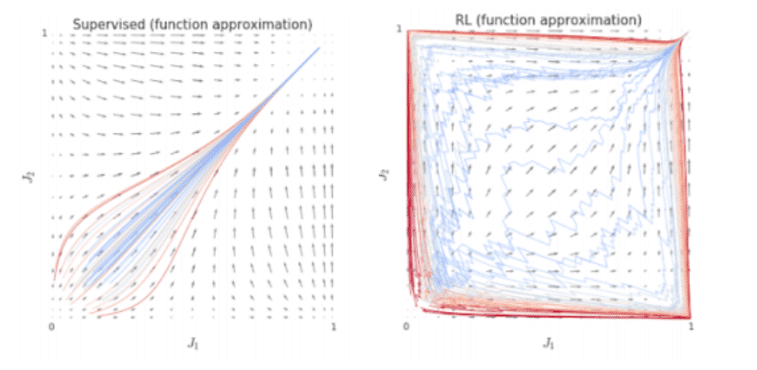The loss function is a sum of J₁+J₂. Basins of attraction show usual trajectories during learning.  Left: Supervised. Right: Reinforcement learning. From [Schaul].

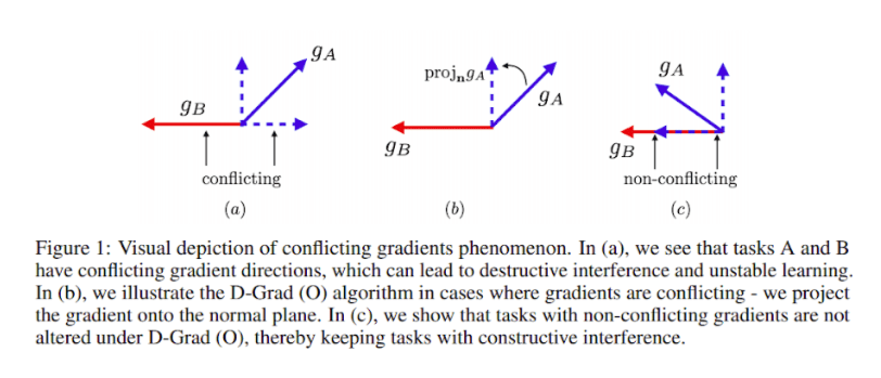
2. Similar explanations for this behavior can come from multi-task learning [Yu]. Here each task has different gradients which could be conflicting and almost canceling each other. [Yu] suggests two different simple approaches to alleviate this problem, one by changing the architecture, second by changing the optimization procedure.

3. High dimensional functions like guessing game with N>10 have (exponentially) more and more saddles compared to local minima or maxima [Dauphin]. All these saddles are accompanied by plateaus of little or no gradient. These saddles and plateaus are strongly linked to the permutation symmetry. Breaking the symmetry in some way removes the plateaus.

4. The currently used loss function (MSE) is not particularly well suited for higher dimensions, where with growing dimensions the distances measured by euclidean norms make less and less sense. The L2 norm is especially problematic. Using the L1 norm instead of MSE showed different behavior in the LSTM meta learner, but not with faster overall convergence or lower error.

LSTM meta learner. Top: L1 loss. Bottom: MSE loss.

F-principle

Quite an important and appreciated feature of supervised deep learning methods is the frequency principle (F-principle) [Zhi-Qin]. F-Principle means that DNN usually solves the low frequencies in the problem first and higher frequencies later. This is a rather peculiar behavior; usual numerical algorithms like Jacobi or Gauss-Seidel methods have the opposite behavior – high-frequency errors are smoothed first. Multi-grid methods are usually used to solve this issue. F-principle is used to explain the surprisingly good generalization of DNNs. 

[Rabinowitz] showed that there is a strong difference between learning in supervised learning and meta-learners. Meta learners do not follow F-principle, but rather learn to solve all the frequencies at the same time.

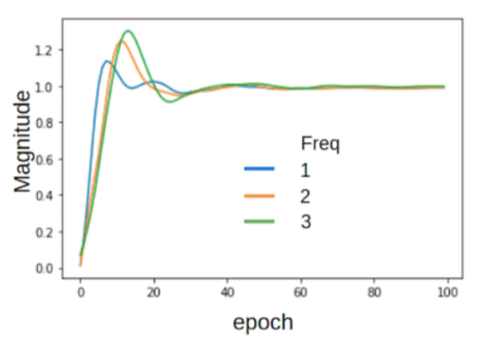
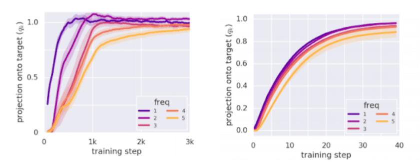Each ‘frequency’ is converged when the magnitude is close to 1.0. Left: Supervised learning, lower frequencies are solved first. Right: Meta-learning, all the frequencies are solved at the same time.

How does the F-principle apply to Badger?

A similar task to the guessing game is used. Guess 41 numbers y _i, these numbers are not random but 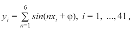where are samples and φ is a random phase shift (the same for all y). The question is always following. Each frequency is correctly solved when the corresponding amplitude reaches one. We want to know if the frequencies reach it in some particular order or all at the same time or in random order.

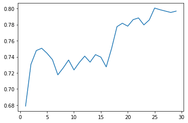
Supervised LSTM (not a Badger), hidden_size=64, 1 layer

• F-principle holds, lower frequencies are solved first.

LSTM, supervised learning

LSTM meta-learner trained with 40 inner loop steps,  hidden_size=64, 1 layer (without GD in the inner loop) 

– no apparent convergence in the inner loop. Lower frequencies are not solved faster but usually with a slightly smaller error.

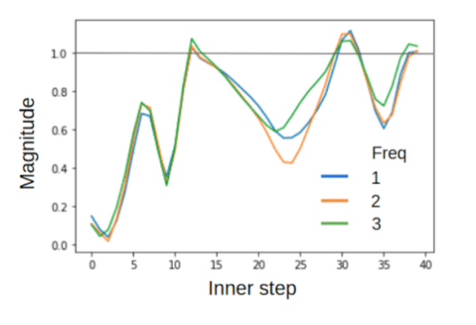
LSTM meta learner with quantized error trained with 100 inner loop steps, hidden_size=64, 1 layer, the error is quantized in 12 bins before passing it to the network 

–  quite a different behavior, with a few distinctive features: 

1. In contrast to meta-lstm with standard meta-lstm, this inner loop converges (last N steps do not change much). The number of converged steps grows with decreasing loss.
2. The F-principle does not apply.
3. Even frequencies usually reach closer to 1, i.e. lower error.

Inner loop step (trained with 100 inner steps), LSTM meta-learner quantized error

Micro-Badger

1. Impossible to converge for too many samples (We had to go from 41 to 11).
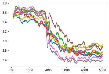
2. F-principle does not apply, some frequencies are solved earlier than others, but the order is rather random.

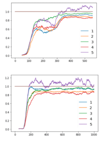Two different runs of microBadger, N=11.

The F-principle does not apply in Badger, but checking it can help you understand how the learning procedure goes. We can conclude that Badger behaves similarly to other meta-learning strategies, thus probably experiencing the same problems. 

Mutual information and (self?)-organization 

Mutual Information

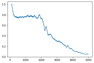
We can observe symmetry breaking while checking the mutual information between the experts (their hidden states) during the learning procedure. As we can see in the following figure (each line is MI between two experts), MI plateaus and then decreases. This gives us evidence that we should make the experts more diverse to speed up the learning and avoid plateaus (or at least have in mind that we need to break the perturbation symmetry somehow). 

Development of Mutual information between pairs of experts, Micro-badger, 14 experts, Dim=4. 5000 outer iterations

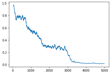
Corresponding error development.

One way to break the first symmetry (effectively remove the first plateau) is to use different weights of each expert in the output, but this approach seems to break an important invariant – the experts are forced to be diverse, this symmetry breaking is not learned. The permutation symmetry does not hold and we force the algorithm to choose a certain path in the function landscape.

Another way around is to compute the hidden state of micro-badger (the RNN) in this way:

hid = 0.5*hid0+0.7*(z_gate*hid + (1-z_gate) * z_val)

Here, hid0 is the previous hid state. Compared to usual 

hid = (z_gate*hid + (1-z_gate) * z_val),

we can see that the update of the hidden state is exponential (e.g. 0.5 + 0.7 > 1). Surprisingly, this does not cause an explosion of hidden states during training. It is unclear how this update breaks the symmetry.

Organization

We can study the organization of the system using information theory [Rosas]. Self-organization of a system is vaguely defined as a system that is subject to:

1. Autonomy: agents evolve in the absence of external guidance.
2. Horizontality: no single agent can determine the evolution of a large number of other agents.

And which generates:

1. Global structure: the system evolves from less to more structured collective configurations.

In our case, we have the external guidance – the loss function and the error that is provided to the experts, this means that we cannot simply talk about self-organization, but rather about guided self-organization [Prokopenko].

We can understand the behavior of the experts with methods from self-organization and information theory. Binding information [Rosas] can be used to explore the level of organization of the behavior of the experts. 

The binding information B quantifies the part of the joint Shannon entropy that is shared among two or more experts and is a complement to the residual entropy (non-shared entropy).

In the case of micro-Badger, binding information grows during the learning, which indicates that the level of organization of the outer loop (outputs of each expert) is growing.

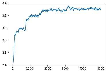
Top: Binding information in micro-Badger – outer loop, 16 experts, 4 links, Dim=4. Bottom: Loss.

What happens during the inner loop? We can check the binding information and we directly see that it does grow as well during the rollout of the inner loop.

Binding information in micro-Badger – inner loop. 

By increasing organization, with decreasing error means that Badger is exploiting the communication between the experts to solve the task. The task could be solved without communication at all (it means without any organization) but Badger takes advantage of the communication when present. We can also see that with higher organization we see lower error, so applying methods that support the organization could be helpful.

We can use other methods (Information decomposition and sharing modes) described in [Rosas] to understand what happens when we add more experts. The analysis shows that the problem is redundancy-dominated (each new expert brings only less and less new information). The opposite is a synergy dominated problem (each new expert brings more and more new information). The former means that there is a number of experts which, if exceeded, do not improve the solution at all but only slow down the whole convergence.

Misc

Topology

Why is the topology of the experts important? We can think of Badger’s inner loop as autonomous differential equations (autonomous ODEs). There is a body of literature describing the topology of the graphs in autonomous ODEs and its effect on convergence. There is a strong incentive to use strongly connected graphs to be sure that each information can reach each expert. Also, the eigenvalues of the Laplacian matrix of the graph play an important role in the convergence speed [Yilun]. 

Transiently chaotic NN

We tested Transiently chaotic neural networks (TCNN) [Zhen]. This recurrent neural network is chaotic at the beginning of the training, but the chaotic behavior should be stabilized during the training. This can help explore the landscape of the function and avoid some saddles. The method behaves like annealing, but deterministic. Unfortunately, it proved to be very difficult to make it converge in the end.

Dynamic Mode Decomposition

Dynamic Mode Decomposition [Schmid] is a dimensionality reduction method of spatio-temporal data. This method tries to find spatial modes of the data and also their behavior – if the mode decays, grows exponentially or fluctuates. We were not able to find these modes in the inner loop because the inner loop behavior does not exhibit any periodic behavior and the method is not useful.

Future

• Use Landscape function analysis (LFA) to quantitatively understand what the functional landscape looks like for different architectures and tasks [Bosman].
• Update architecture as in [Yu]. This could be used to decompose the task and avoid conflicting gradients. To mitigate the problem of conflicting gradients during optimization, [Yu] suggests that we can employ a few very simple architectural changes in the neural network model being learned to encourage the model to have orthogonal gradients. Intuitively, [Yu] simply introduces a particular variant of multiplicative interactions with network activations, which greatly reduces the occurrence of conflicting gradients during optimization.
• Update optimization procedure as in [Yu] or try to use some “saddle avoiding methods” like approximate natural gradients. E.g. [George].
• Explore the use of meta-learning to design better parametric loss functions [Bechtle]. Designing loss function exactly for each problem can speed-up the convergence.
• Explore the effects of using strongly connected topologies, with different eigenvalues of the Laplacian matrix.
• Explore more the application of the chaotic regime with a method similar to [Das].
• Analyze whether adding new experts is redundant or synergetic according to information theory [Rosas].

Conclusion

Why is Badger hard to train? Badger suffers from similar issues that other reinforcement learning or meta-learning algorithms suffer from. The reason for the plateaus and the saddles is similar to RL. F-principle also shows that the learning in Badger is similar to other meta-learning algorithms: the F-principle does not hold. There is an “extra” difficulty connected to the homogeneity of the experts and thus added symmetry. We used Mutual information to explain that only after the experts are more diverse, the plateaus are escaped. Binding information on the other hand also shows that the organization of the inner and outer loop is increasing in time. Two different ways to remove the first plateau are suggested (different weights of the experts and exponential hidden state update).

The one (partial) way out of this could consist of a few steps: 

1. Learn how the landscape looks like (LFA), learning this can help to understand how the changes in loss or architecture influenced the landscape.
2. Learn how to make exploration easier (meta-learned loss function). 
3. Apply “saddle escaping” optimization (natural gradient). 
4. Apply some small architecture changes [Yu].

Another way could be to learn differently, e.g. try to reframe Badger as a “guided self-organization” algorithm and use techniques like versions of Hebbian networks [Der].

Literature

[Rosa] Rosa, et al. BADGER: Learning to (Learn [Learning Algorithms] through Multi-Agent Communication), 2019.

[Yu] Multi-Task Reinforcement Learning without Interference, 2019.

[Schaul] Ray Interference: a Source of Plateaus in Deep Reinforcement Learning, 2019.

[Dauphin] Dauphin, et al. Identifying and attacking the saddle point problem in high-dimensional non-convex optimization, 2014.

[Rabinowitz] Rabinowitz, Meta-learners’ learning dynamics are unlike learners’, 2019.

[Zhi-Qin] Zhi-Qin, et al. Frequency principle: Fourier analysis sheds light on deep neural networks, 2018.

[Rosas] Rosas, et al., An Information-Theoretic Approach to Self-Organisation: Emergence of Complex Interdependencies in Coupled Dynamical Systems, 2019.

[George] George, et al. Fast Approximate Natural Gradient Descent in a Kronecker-factored Eigenbasis, 2018.

[Yilun] Yilun, Finite-time consensus for multi-agent systems with fixed topologies, 2012.

[Bechtle] Bechtle, Meta Learning via Learned Loss, 2019.

[Zhen] Zhen, et al. A study of the transiently chaotic neural network for combinatorial optimization, 2002.

[Bosman] Bosman, Fitness Landscape Analysis of Feed-Forward Neural Networks, 2012.

[Das] Das, Stability and chaos analysis of a novel swarm dynamics with applications to multi-agent systems, 2014.

[Prokopenko] Prokopenko, Guided self-organization, 2009.

[Der] Der, In Search for the Neural Mechanisms of Individual Development: Behavior-Driven Differential Hebbian Learning, 2016.

[Barakova] Barakova,  Learning reliability: a study on indecisiveness in sample selection, 1999.

[Schmid] Schmid, Dynamic mode decomposition of numerical and experimental data, 2010.

Collaborate with us

If you are interested in Badger Architecture and the work GoodAI does and would like to collaborate, check out our GoodAI Grants opportunities or our Jobs page for open positions!

For the latest from our blog sign up for our newsletter.